Calculating Industrial Computer Payback Period: A Complete Guide

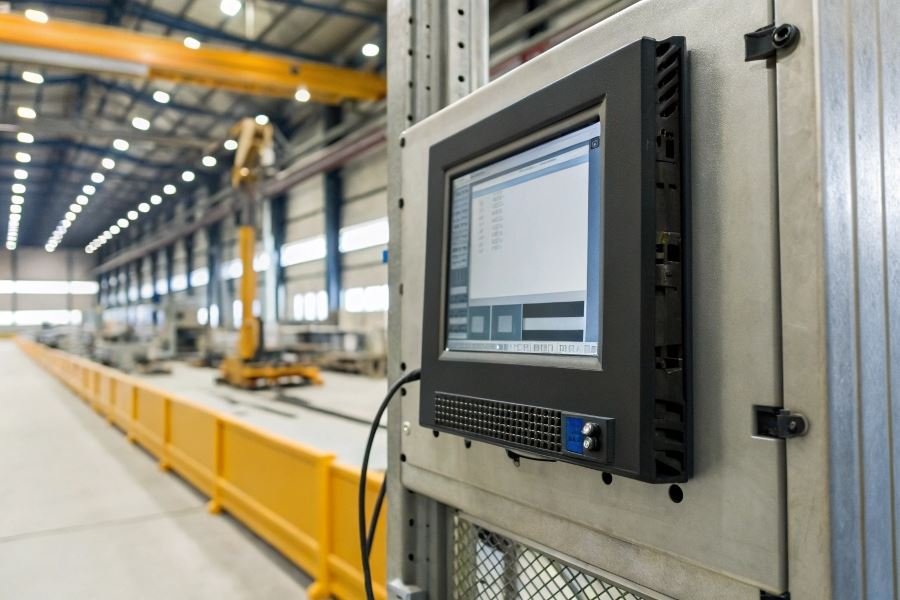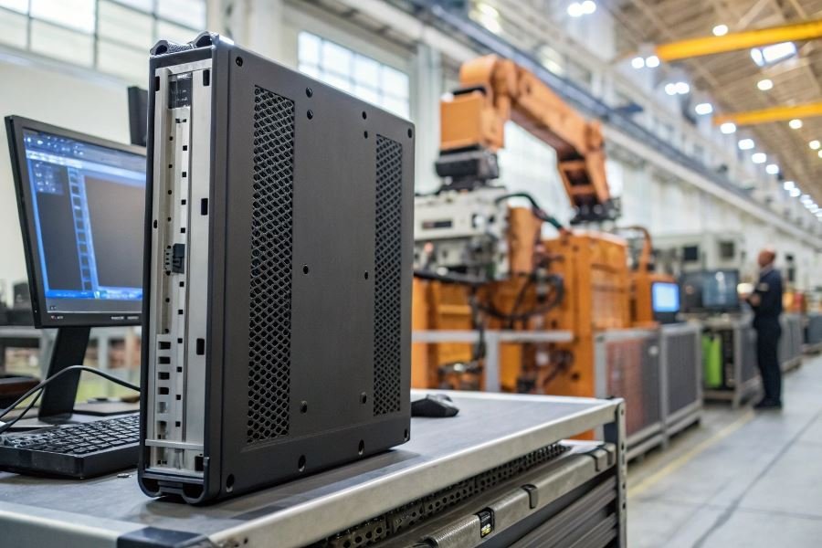
Ever watched $250,000 in hardware get installed on your factory floor and wondered, “When exactly will this investment start paying for itself?” You’re not alone. The payback period calculation isn’t just another financial metric—it’s the compass that guides smart industrial technology investments.

The payback period represents the time required for an industrial computer implementation to recoup its initial investment through generated benefits. Unlike consumer technology that might be replaced on a whim, industrial computing solutions demand rigorous financial justification. A manufacturing plant in Michigan recently discovered their $175,000 investment in ruggedized computing systems paid for itself in just 11 months—far outpacing their projected 18-month timeline.

Before calculating your payback period, gather these critical financial metrics:

• Total implementation costs (hardware, software, installation, training)
• Projected monthly or annual savings (labor reduction, increased throughput)
• Maintenance expenses over the expected lifespan
• Opportunity costs of alternatives or doing nothing

Beyond simple division: The complete ROI picture

While basic payback calculation involves dividing costs by annual savings, sophisticated evaluations incorporate:

• Time value of money (a dollar today is worth more than tomorrow)
• Risk assessment factors unique to your industry
• Productivity gains that compound over time
• Downtime reduction value specific to your operation

The most successful implementations track both tangible metrics (energy savings, labor reduction) and intangible benefits (improved quality, enhanced safety) to create a comprehensive ROI evaluation that justifies the initial investment many times over.

Calculating Industrial Computer Payback Period: A Practical Guide

When investing in industrial computing solutions, the bottom line matters. Smart business decisions require understanding exactly when your investment will start paying for itself. Let’s dive into the nuts and bolts of how to calculate the payback period when implementing industrial computers in your manufacturing or industrial environment.

Tallying the True Implementation Costs

The first step in any payback analysis requires brutal honesty about what you’re spending. Industrial computer implementation costs extend far beyond the sticker price of the hardware.

Hardware costs include not just the industrial PCs themselves (typically 1, 500−5,000 per unit depending on specifications), but also peripherals like ruggedized displays, specialized input devices, mounting hardware, and networking equipment. A mid-sized factory floor might require 10-15 units, immediately pushing hardware costs into the $30,000+ range.

Software investments often match or exceed hardware expenses. This includes:

• Operating system licenses
• Specialized industrial control software
• SCADA systems
• Custom application development
• Integration middleware

Don’t overlook installation expenses. Professional installation for industrial-grade systems typically runs 15-20% of hardware costs, covering proper mounting, electrical work, network configuration, and environmental protection.

Training costs represent the final major implementation expense. Factory staff require comprehensive training on new systems, which might include:

Training Type	Typical Cost	Duration
Operator Training	$500-1,000/person	2-3 days
Maintenance Training	$1,200-2,500/person	1 week
Administrator Training	$3,000-5,000/person	1-2 weeks

Quantifying Annual Benefits and Savings

The exciting part comes when identifying the tangible benefits your industrial computer implementation delivers. These typically fall into several categories:

Productivity improvements often represent the largest benefit. Modern industrial computers from manufacturers like Dell Industrial or Advantech can reduce production cycle times by 15-30% through automation and real-time monitoring.

Reduced downtime delivers immediate ROI. Industrial computers with predictive maintenance capabilities can slash unplanned downtime by 30-50%, a massive benefit when considering that downtime costs average 5, 000−10,000 per hour in many manufacturing environments.

Quality improvements translate directly to bottom-line benefits:

• Reduced scrap rates (typically 5-15% improvement)
• Fewer warranty claims
• Higher customer satisfaction
• Premium pricing opportunities

Labor efficiency gains come from automation of manual processes and better resource allocation. Many implementations report 20-25% labor efficiency improvements.

Applying the Payback Period Formula

With costs and benefits quantified, calculating the payback period becomes straightforward. The basic formula is:

Payback Period = Total Implementation Cost ÷ Annual Cost Savings

Let’s work through a practical example:

A medium-sized manufacturing operation implements industrial computers with:

• Hardware costs: $75,000
• Software and integration: $90,000
• Installation: $15,000
• Training: $20,000
• Total investment: $200,000

Annual benefits include:

• Productivity gains: $85,000
• Reduced downtime: $60,000
• Quality improvements: $40,000
• Labor efficiency: $35,000
• Total annual benefit: $220,000

Applying our formula: $200,000 ÷ $220,000 = 0.91 years, or approximately 11 months.

This sub-one-year payback period represents an excellent investment opportunity, especially considering industrial computers typically have a 5-7 year operational lifespan, meaning over 6 years of pure financial benefit after the initial payback period.

Beyond Basic Payback: Advanced Financial Analysis for Industrial Computing

The True Cost Picture: Depreciation and Maintenance

When calculating the payback period for industrial computers, looking only at purchase price versus immediate savings creates a dangerously incomplete picture. Depreciation schedules dramatically affect your true ROI timeline. Industrial computers typically depreciate over 3-5 years for accounting purposes, but their actual useful life often extends to 7-10 years in well-maintained environments.

Maintenance costs follow a predictable pattern: minimal in years 1-2 (typically covered by warranty), increasing by approximately 15-20% annually thereafter. A $5,000 industrial computer might require just $200 in maintenance during year three, but climb to $500+ by year five.

Consider this maintenance cost progression for a typical industrial computing implementation:

Year	Maintenance Cost	Cumulative Cost	Notes
1-2	$0-100	$0-100	Warranty coverage
3	$200-300	$200-400	Basic maintenance
4	$300-400	$500-800	Component replacements begin
5	$400-600	$900-1,400	Significant updates needed
6+	$500-800+	$1,400-2,200+	Approaching replacement threshold

These escalating costs must be factored into your payback calculations. The formula becomes:

Payback Period = (Initial Investment + NPV of Maintenance) ÷ (Annual Benefits – Annual Depreciation)

Risk Factors and Sensitivity Analysis

Every industrial computer implementation carries unique risks that can extend payback periods. Sensitivity analysis reveals how vulnerable your projections are to changing conditions.

The three critical variables to stress-test:

1. Downtime frequency – Even a 99.9% uptime guarantee means 8.76 hours of downtime annually
2. Implementation timeline slippage – Each month of delay typically erodes 5-8% of first-year benefits
3. Staff adaptation curve – Productivity often dips 10-15% during the first 60-90 days before improvements begin

Create multiple scenarios by adjusting these variables. A robust implementation plan should withstand a 20% negative variance in any single factor while still delivering acceptable payback periods.

Beyond Payback: Comprehensive Financial Evaluation

Payback period alone provides insufficient guidance for industrial computing investments. Supplement with these metrics for deeper insight:

Net Present Value (NPV) calculates the current value of all future cash flows, accounting for the time value of money. A positive NPV indicates a profitable investment beyond just breaking even.

Internal Rate of Return (IRR) reveals the annual growth rate your investment generates. Compare this against your company’s hurdle rate (minimum acceptable return) for context.

Total Cost of Ownership (TCO) captures all direct and indirect costs over the solution’s lifecycle, including:

Cost Category	Typical Percentage of TCO	Often Overlooked Elements
Hardware	35-40%	Specialized peripherals, backup systems
Software	15-20%	Annual license fees, security updates
Implementation	10-15%	Production disruption, testing
Maintenance	20-25%	Preventive maintenance, not just repairs
Training	5-10%	Ongoing training for new staff
Energy	5-10%	Cooling requirements, power conditioning

The most successful industrial computing implementations achieve payback within 18-24 months while delivering positive NPV and IRR exceeding the company’s hurdle rate by at least 15%.